Exercise: four questions, four charts

Session 5 — Applied Data Science 2026

Author

Affiliation

Claudius Gräbner-Radkowitsch

EUF and JKU

NoteThe setting

The hotel group from sessions 1 to 3 knows Vienna inside out. Now it is looking at the rest of Europe, and the board has questions: what a night costs, which cities are cheap, whether location matters everywhere, and when the market is quiet.

But: Nobody on the board has time to read tables. Thus, every answer you give today has to be a chart.

Alone or in pairs.

Your task: Create session05.qmd in your project and answer the questions below in order, one chart each. Before every chart, write one sentence that says what goes where — “price on the x axis, one bar per price range” — and only then write the code. If you cannot write the sentence, the code will not help you.

ImportantStart here

Copy both CSV files from the session page into your project’s data/ folder. Then create session05.qmd with this setup chunk:

```{r}
#| label: setup
#| include: false
library(tidyverse)  # includes ggplot2 and forcats
library(scales)     # axis labels in euros
library(here)

i_am("session05.qmd")

prices   <- read_csv(here("data", "hotels-europe_price.csv"))
features <- read_csv(here("data", "hotels-europe_features.csv"))
```

Every path goes through here(), as since session 3.

1 Q1 — Two files, one table

Neither file can answer anything on its own. Build the table you will plot from: hotels only, on one date — a weekday night in November 2017 — with each hotel’s features attached. You may start from this:

nov <- prices |>
  filter(year == 2017, month == 11, weekend == 0)

hotels <- nov |>
  ___(features, by = "___") |>
  filter(city == city_actual, accommodation_type == "Hotel") |>
  mutate(star_tier = factor(floor(stars + 0.5), levels = 1:5,
                            labels = paste(1:5, "stars")))

Fill in the two blanks. Then report how many rows you have after each of the three steps: the date filter, the join, and the second filter(). Write those numbers in your text, as inline code.

TipHint

The join is inner_join(), and the column both files share is hotel_id. nrow(nov) gives you the first number.

If the join changed the number of rows, something is wrong — every price row belongs to exactly one hotel. Check it before you go on.

NoteWhat city == city_actual is for

city is the city a hotel was listed under on the website; city_actual is where it actually is. Some hotels listed under “Vienna” are in a suburb — you met them in session 1. We keep only hotels that are where they claim to be.

2 Q2 — What does a night cost?

Board: “What does a hotel night in Europe typically cost?”

One numerical variable, so: one distribution. Draw a histogram of price across all hotels in hotels.

1. Describe in one sentence what you see. Where are most hotels, and how much of the chart are they using?
2. Add scale_x_log10(). Describe again.
3. The log axis labels are still bare numbers. Replace them with euros and with breaks a reader can use.

TipHint

 scale_x_log10(____ = c(25, 50, 100, 200, 400, 800),
               ____ = label_number(prefix = "€"))

On this axis, each step is a doubling. Write down what that means for how far apart €50 and €100 are, compared with €400 and €800.

4. Find the most expensive hotel in the data with slice_max(hotels, price). Does it look like a real price? Where is it on the linear chart, and where on the log chart?

TipHint

ggplot(data = hotels, mapping = aes(x = price)) +
  geom_histogram(bins = 50) +
  labs(x = "Price per night", y = "Number of hotels")

Try a few values of bins — 20, 50, 100. The number of bins is a choice, and it changes what the chart seems to say.

NoteWhy “typical” changes meaning on a log axis

On a linear axis, a hotel that charges €50 more is the same distance away whether it starts from €50 or from €500. On a log axis, a hotel that charges twice as much is the same distance away, wherever it starts.

Prices behave like the second kind. A hotel can charge ten times the median, but none can charge less than nothing — so the long tail only runs one way, and the differences that matter are ratios. That is why the log chart looks roughly symmetric and the linear one does not.

3 Q3 — Which cities are cheap?

Board: “Where is it cheap, where is it expensive — and how much do the cities differ?”

A comparison between groups. Keep eight cities:

eight <- hotels |>
  filter(city %in% c("Amsterdam", "Berlin", "Budapest", "Lisbon",
                     "London", "Paris", "Prague", "Rome"))

Draw one boxplot per city, with the cities on the y axis and price on a log scale on the x axis. Then:

1. Order the cities by their median price, so the chart reads from cheap to expensive — fct_reorder() does it inside aes().
2. Roughly how many times more expensive is the median hotel in the most expensive city than in the cheapest? Read it off the chart, then check it with summarise().
3. How many hotels is each box based on? Find out, and write the smallest one in your text.

TipHint

ggplot(data = eight, mapping = aes(x = price, y = fct_reorder(city, price))) +
  geom_boxplot() +
  scale_x_log10(___) +
  labs(x = ___, y = NULL)

fct_reorder(city, price) turns city into a factor ordered by the median of price in each city.

Why the y axis? Because city names are long, and on the x axis they would overlap. Swapping x and y is one of the cheapest readability gains there is.

NoteWhy a boxplot and not a bar of the averages?

A bar of the median shows one number per city. A boxplot shows the median and how spread out the prices are around it — and in some of these cities the spread is as interesting as the level. If the board asks “is Paris expensive?”, the honest answer is about the whole box.

4 Q4 — Does location matter everywhere?

Board: “In Vienna, central hotels charge more. Is that true in every city?”

A relationship between two numbers — distance and price — so: a scatter plot. Use four cities:

four <- hotels |>
  filter(city %in% c("Amsterdam", "Budapest", "Lisbon", "Prague"))

1. Write the mapping sentence first. Then draw distance against price, with price on a log scale.
2. Many points sit on top of each other. Make them semi-transparent.
3. Add facet_wrap(~ city). What does that line do — in terms of the grammar, which part of the chart has it added?
4. Add a trend line with geom_smooth(se = FALSE). In which of the four cities does the centre matter most? Least?
5. Now remove the facets and map colour = city instead. Which version answers the board’s question better, and why?

TipHint

ggplot(data = four, mapping = aes(x = distance, y = price)) +
  geom_point(alpha = 0.3) +
  geom_smooth(se = FALSE) +
  scale_y_log10(labels = label_number(prefix = "€")) +
  facet_wrap(~ city) +
  labs(x = "Distance to city centre (km)", y = "Price per night")

alpha runs from 0 (invisible) to 1 (solid). Notice that it is outside aes() — see the optional task (a) below for why that matters.

5 Q5 — Rating or stars?

Board: “Do guests pay more for a better-rated hotel? Or is that just the stars talking?”

The confounding question from session 1, now with a third variable on the chart. Take the three- and four-star hotels in Paris:

paris <- hotels |>
  filter(city == "Paris", star_tier %in% c("3 stars", "4 stars"))

1. Draw rating against price (log scale), and map colour to star_tier.
2. Add geom_smooth(method = "lm", se = FALSE). You get one line per colour — why?
3. Within each star tier, do better-rated hotels charge more? Is the answer the same for both tiers?
4. Try facet_wrap(~ star_tier) instead of colour. Which version makes the comparison easier?

TipHint

A mapping in ggplot() applies to every layer, so the colour mapping also splits geom_smooth() into one line per star tier. That is usually what you want — and occasionally a surprise.

If ggplot warns that it removed rows, read the warning: some hotels have no rating, and your chart then shows fewer hotels than your table.

6 Q6 — When is a weekend cheapest?

Board: “We want to run a weekend promotion. When are prices low anyway?”

A change over time: a line chart. The data has weekend prices for seven months. Build the table:

weekends <- prices |>
  filter(weekend == 1) |>
  inner_join(features, by = "hotel_id") |>
  filter(city == city_actual, accommodation_type == "Hotel",
         city %in% c("Amsterdam", "Budapest", "Lisbon", "Prague")) |>
  group_by(city, year, month) |>
  summarise(n = n(), median_price = median(price), .groups = "drop") |>
  mutate(date = make_date(year, month))

1. Draw date against median_price, one line per city.
2. Add points on top of the lines. Why is that a good idea here?
3. One month is missing from the data entirely. Which one, and what does your line claim about it anyway?
4. Look at the n column. Is every point based on a similar number of hotels?
5. Which month would you recommend for the promotion?

TipHint

For lines, the grouping comes from colour:

ggplot(data = weekends, mapping = aes(x = date, y = median_price, colour = city)) +
  geom_line() +
  geom_point() +
  scale_x_date(date_breaks = "1 month", date_labels = "%b")

The last line puts a label on every month instead of every quarter.

Should the y axis be on a log scale here as well? Try it, and decide which question each version answers better.

7 Q7 — Reverse engineering

Here is a chart somebody made from hotels. Write the code that produces it.

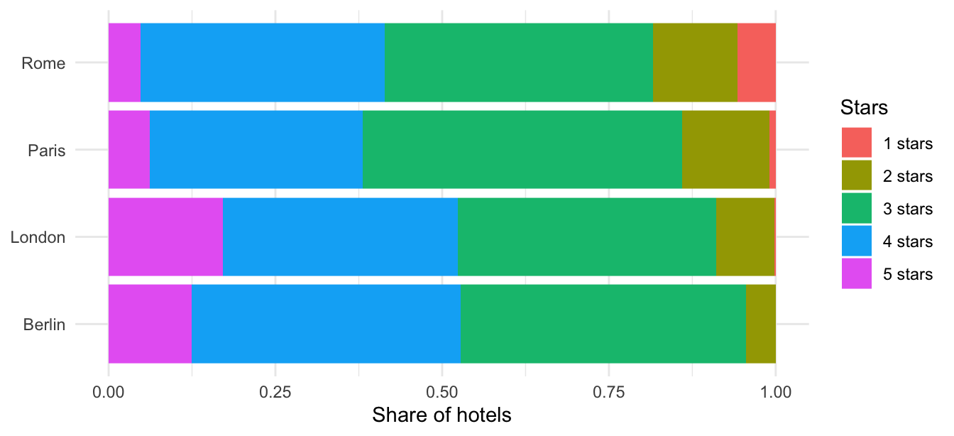
Start by writing the mapping sentence: what is on each axis, what does the colour show, and what has been done to the bars? Then write the code.

TipHint

• The four cities are Berlin, London, Paris and Rome. Hotels without a star rating have been dropped.
• There is no x in the mapping. geom_bar() counts rows by itself — that count is a computed variable, the stat part of the grammar.
• The bars all have the same length. Look at the position argument of geom_bar().
• The grey background is gone: one of the built-in theme_*() functions.

8 The checklist

Before you say you are done:

• a mapping sentence above every chart
• every axis says what it shows, with the unit — “Price per night”, not price
• every log axis is labelled in euros, not in powers of ten
• n reported for the joined table and for the smallest group you plotted
• the document renders, from a restarted R session

9 If you finish early

9.1 a) Mapping or setting?

Run this and explain what went wrong:

ggplot(data = four, mapping = aes(x = distance, y = price, colour = "steelblue")) +
  geom_point()

The points are not steel blue, and there is a legend that says "steelblue". Fix it so the points really are steel blue. Then write one sentence on the difference between putting colour inside and outside aes().

9.2 b) The four-night trap

So far you only used one date. Join all rows of the price file to the features and draw a histogram of price on a log scale. It looks perfectly reasonable.

Now map fill to factor(nnights). What has been hiding in that histogram, and why would a chart of “average price by month” built from all rows be wrong?

9.3 c) Nine and a half thousand points

Draw distance against price (log scale) for all hotels in hotels. Even with alpha it is a cloud. Replace geom_point() with geom_bin2d() and explain what the chart now shows instead of points.

9.4 d) All of Europe

Repeat Q3 for every city in hotels. Where does Vienna rank? How many hotels does the smallest city have — and would you show that box to the board?