Where should we build?

A briefing on four-star hotel pricing in Vienna · Exemplary solution, Session 3

NoteHow to read this document

Sections 1 to 4 are the deliverable: the briefing itself, written the way a report should be written. Read those as the standard expected — including the interpretation sentences, which matter as much as the code.

Section 5 onwards is commentary: how the requirements on the exercise sheet were met, and full answers to the four optional tasks. In a real submission that part would not be there.

This is one potential answer, not the answer.

WarningOne deliberate deviation: i_am() and here()

The exercise sheet asks you to open with i_am("session03.qmd") and read the data with here("data", "hotels-vienna.csv"), and you should. This file does neither, because every session folder on this website is self-contained — the data sits next to the document so the pair can be downloaded and used without a project around them. There is no project root here to declare.

In your project there is one .Rproj at the root and several documents inside it. That is exactly the situation those two lines exist for. Use both: i_am() once at the top, here() in every path. Report 1 asks for both.

library(tidyverse)  # Standard packages for data transformation
library(flextable)  # For printing nice tables in Quarto

hotels <- read_csv("data/hotels-vienna.csv")

1 The question

The board is considering a four-star property in Vienna and wants to know how much more a central hotel can charge its guests per night. This briefing answers that from the prices of the hotels already operating in the city.

2 The data and what was removed

The data covers 428 properties in and around Vienna, priced for one night in November 2017 (Békés and Kézdi 2021).

hotels_clean <- hotels |>
  filter(city_actual == "Vienna", price < 1000) |>
  mutate(
    band = cut(distance, c(-0.1, 1, 2, 3, 100),
               labels = c("<1 km", "1-2 km", "2-3 km", ">3 km")),
    star_tier = factor(floor(stars + 0.5), levels = 1:5,
                       labels = paste(1:5, "stars"))
  )

only_hotels <- hotels_clean |>
  filter(accommodation_type == "Hotel")

Three restrictions, each with a reason:

1. 10 properties are not in Vienna at all — Schwechat is the airport — so “distance to the city centre” does not mean the same thing for them.
2. One three-star hotel is priced at €1,012, against €806 for the next most expensive property in the whole dataset. Almost certainly a data-entry error.
3. Apartments are priced per unit rather than per room, so they are not comparable with hotel rooms. The briefing therefore uses the 253 hotels among the 417 remaining properties.

Half-star ratings were rounded up into five tiers, so that the groups are large enough to compare.

3 What four-star hotels charge

four_star <- only_hotels |>
  filter(star_tier == "4 stars") |>
  group_by(band, .drop = FALSE) |>
  summarise(n = n(), median_price = median(price), .groups = "drop")

ft(four_star)

Table 1: Four-star hotels in Vienna: number of properties and median price per night, by distance to the city centre.

band	n	median_price
<1 km	63	138.0
1-2 km	39	95.0
2-3 km	12	88.5
>3 km	11	81.0

Of the 125 four-star hotels in the sample, the 63 within one kilometre of the centre charge a median of €138 per night. The 39 between one and two kilometres out charge €95 — a difference of €43 per night, or 45.3%.

Beyond two kilometres the gradient nearly disappears: €88.50 in the two-to-three kilometre band and €81 further out, a gap of only €7.50 across a whole additional kilometre. Figure 1 shows the shape.

ggplot(four_star, aes(x = band, y = median_price)) +
  geom_col(fill = "#69AACD") +
  geom_text(aes(label = eur(median_price, 0)), vjust = -0.4, size = 3.5) +
  scale_y_continuous(expand = expansion(mult = c(0, 0.12))) +
  labs(
    x = "Distance to city centre",
    y = "Median price per night (EUR)",
    title = "The premium is concentrated in the first kilometre"
  ) +
  theme_classic()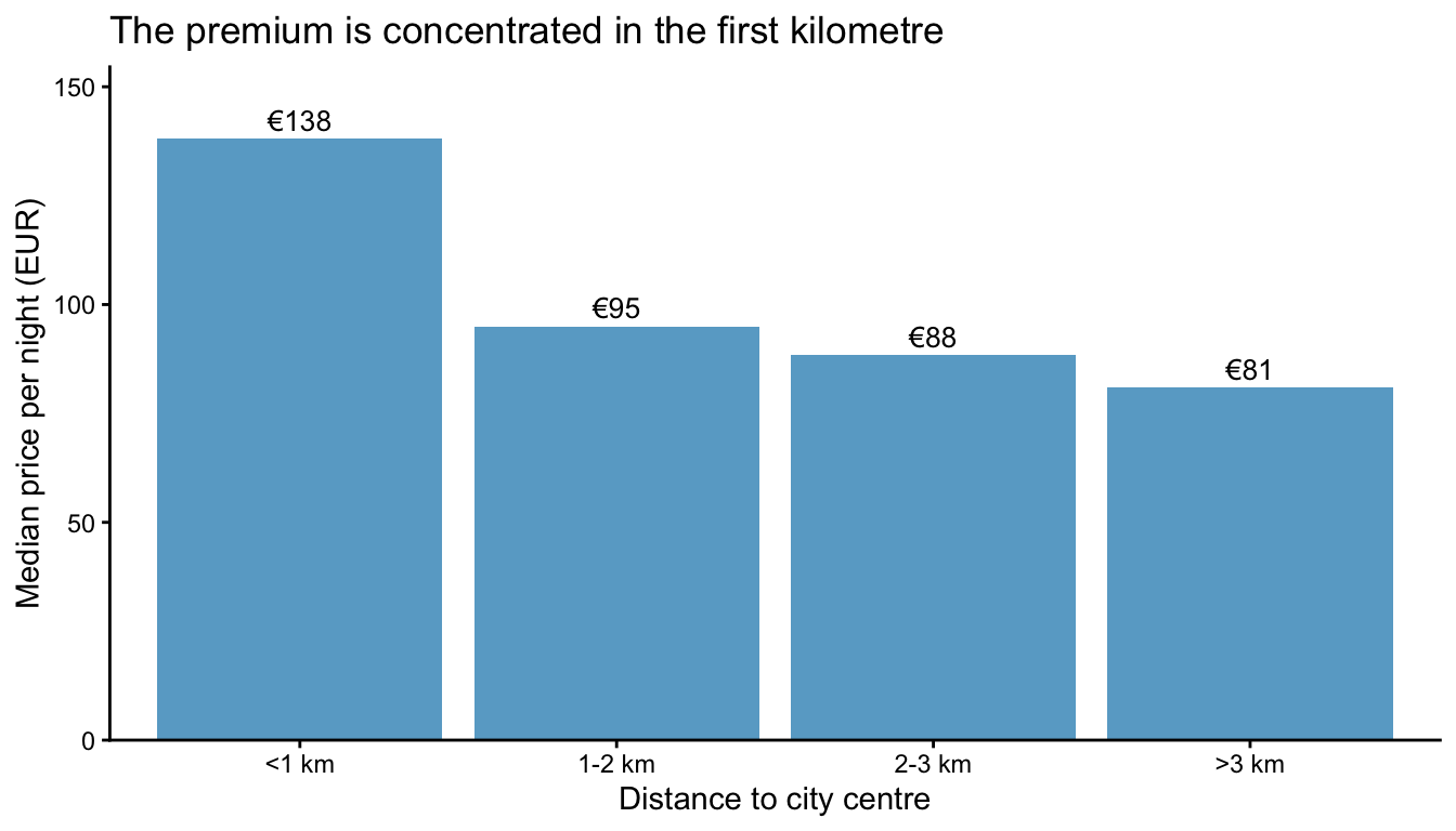

Figure 1: Median price of four-star hotels by distance to the city centre.

4 What this does and does not say

Among four-star hotels currently operating in Vienna, those within a kilometre of the centre charge about €43 more per night than those one to two kilometres out. Beyond that, distance is close to irrelevant: a site three kilometres out and a site five kilometres out face nearly the same market.

ImportantThe phrasing the board will misread if you let them

The honest sentence is “central four-star hotels charge about €43 more per night.”

The tempting sentence is “a central location is worth €43 per night.” We have not shown that. Central hotels may differ from outlying ones in ways this data does not record — the building, the room sizes, the management. Moving our hotel a kilometre inward would not automatically add €43 to what we can charge.

A difference between existing hotels is not the effect of a decision. Session 8 is about the gap between those two, and it is the distinction the exam asks you to make.

And note which side of the business this number lives on. It is what hotels charge their guests — revenue. What a central plot costs the group to buy or lease is a different number, and there is nothing about it in this data. A premium on the revenue side is not by itself a reason to pay for the location.

The practical implication is a threshold rather than a gradient: either pay for the first kilometre, or stop paying for proximity at all. A site at 1.5 kilometres carries most of the cost of being central and little of the extra revenue.

5 How the requirements were met

NoteQ1 — the header

---
title: "Where should we build?"
author: "Your Name"
date: "2026-09-28"
format:
  html:
    toc: true
    number-sections: true
execute:
  echo: true
  warning: false
  message: false
bibliography: references.bib
---

One entry under format:, which is all the exercise asks for. execute: applies to every chunk, and that is what keeps tidyverse’s start-up message out of the finished document.

number-sections: true is not decoration. Without numbered sections there is nothing for a cross-reference to a section to point at.

In your project bibliography: is simply references.bib. This file says ../../references/references.bib because the website keeps one shared bibliography two folders up.

This document also carries a pdf: entry, because it answers optional task (d) in Section 9. You do not need one.

NoteQ2 — the structure

The four ## sections of this briefing are the answer to Q2, and their order is the point:

1. The question — what was asked, in one short paragraph
2. The data and what was removed — what the numbers rest on, and what was thrown away, before any finding is claimed
3. What four-star hotels charge — the finding, with its table and figure
4. What this does and does not say — the caveat, stated by the author rather than discovered by the reader

That is a general shape for a short analytical report, and it is worth keeping: question → data → finding → limits. A reader who only has two minutes reads sections 1 and 4 and is not misled.

The key finding is in bold in section 4, and the three restrictions in section 2 are a numbered list because they are three separate decisions, each needing its own justification — not one paragraph of prose with three clauses.

NoteQ3 — every number inline

Every number in section 3 is computed; not one of them is typed. The pattern throughout is: compute once into a named object, then refer to it.

The `r n_in` within one kilometre of the centre charge a
median of `r eur(med_in)` per night.

Pulling the values out into n_in, med_in and so on in an include: false chunk is worth the extra three lines: the alternative is four_star$median_price[four_star$band == "<1 km"] written out five times in the middle of a sentence, which nobody can read.

The eur() helper does the formatting. Without it the text would say €138.00 in some places and €138 in others, depending on what the median happened to be.

NoteQ4 and Q5 — cross-references

Table 1 and Figure 1 are both produced by chunks carrying a label: with the right prefix and a caption:

#| label: tbl-fourstar
#| tbl-cap: "Four-star hotels in Vienna: ..."

#| label: fig-bands
#| fig-cap: "Median price of four-star hotels ..."

Note that Figure 1 carries both a caption and a title inside labs(). The caption says what the reader is looking at; the title says what to conclude. In a briefing you want both.

If you saw ?fig-bands in your output, that is the failure from the slides: the render succeeded, nothing appeared in the log, and the reference found nothing to point at. Either the caption is missing — a figure without fig-cap is not registered as a figure at all — or the label does not begin with fig- / tbl-. It is the one error in this session that you can only catch by reading the rendered page.

NoteQ6 — the citation

bibliography: in the header, [@bekes2021data] in section 2, and the ::: {#refs} block at the very end. Only the works actually cited appear — which is the main practical reason to use a .bib file rather than typing references by hand.

NoteQ7 — reproducibility

This document renders from a restarted session. The things that make that true:

• every package is loaded in the setup chunk, in the document
• every object it uses is created in the document
• the data is read from a file — in your version, through here(), with i_am() above it
• no setwd(), no install.packages(), nothing interactive like View()

The test is the one from the slides: Session → Restart R, then Render. If a chunk fails after that, the object or package it wanted lives in your console and not in the document — Objekt 'x' nicht gefunden, or object 'x' not found if your R is set up in English.

The one thing you cannot check by rendering it yourself is whether it works on another machine. Only somebody else’s laptop tells you that, which is why the exercise asks you to swap folders.

6 Optional task (a): the messy import

hotels-vienna-messy.csv is the same data as a German Excel export. Four things are wrong with it at once.

6.1 What it looks like before you touch it

naive <- read_csv("data/hotels-vienna-messy.csv", show_col_types = FALSE)
dim(naive)

[1] 428   1

1 column. The whole file has been read as a single text column, because read_csv() splits on commas and this file has none — it uses semicolons.

WarningWhy R did not warn you properly

It did, quietly: a parsing-issues warning that most people scroll past. The dim() is the real signal. Always check the dimensions of anything you just imported. 428 × 1 is obviously wrong for a file with nine fields per line; 428 × 9 would have been obviously right.

6.2 Fixing it

library(janitor)  # For clean_names()

messy <- read_csv2(
  "data/hotels-vienna-messy.csv",
  locale = locale(encoding = "ISO-8859-1",
                  decimal_mark = ",",
                  grouping_mark = "."),
  na = c("", "k.A."),
  show_col_types = FALSE
) |>
  clean_names()

glimpse(messy)

Rows: 428
Columns: 9
$ hotel_id               <dbl> 21894, 21897, 21901, 21902, 21903, 21904, 21906…
$ stadt                  <chr> "Wien", "Wien", "Wien", "Wien", "Wien", "Wien",…
$ stadtteil              <chr> "17. Hernals", "17. Hernals", "Alsergrund", "Al…
$ unterkunftsart         <chr> "Apartment", "Hotel", "Hotel", "Hotel", "Hotel"…
$ preis_pro_nacht_in_eur <dbl> 81, 81, 85, 83, 82, 229, 103, 150, 80, 153, 60,…
$ sterne                 <dbl> 4.0, 4.0, 4.0, 3.0, 4.0, 5.0, 4.0, 4.0, 2.0, 3.…
$ entfernung_zentrum_km  <dbl> 2.7, 1.7, 1.4, 1.7, 1.2, 0.9, 0.9, 1.0, 0.7, 1.…
$ gastebewertung         <dbl> 4.4, 3.9, 3.7, 4.0, 3.9, 4.8, 3.9, 4.6, 3.5, NA…
$ anzahl_bewertungen     <dbl> 36, 189, 53, 55, 33, 25, 57, 161, 50, NA, 203, …

Four separate problems, four arguments:

Problem in the file	What fixes it
Semicolons between fields	read_csv2() instead of read_csv()
Decimal comma, full stop for thousands	decimal_mark = ",", grouping_mark = "."
Umlauts stored as ISO-8859-1, not UTF-8	locale(encoding = "ISO-8859-1")
k.A. written where a rating is missing	na = c("", "k.A.")
Column names with spaces, brackets, umlauts	janitor::clean_names()

ImportantThe k.A. problem is the dangerous one

The other three fail loudly. This one fails silently: one non-numeric entry anywhere in a column and R reads the entire column as text.

Without na = c("", "k.A."), gastebewertung arrives as character. Then mean(rating) returns an error you will blame on something else, or — worse — arrange(rating) sorts your hotels alphabetically and returns "3,9" before "4,0" before "k.A.", and nothing warns you at all.

This is exactly the "240" + 10 problem from session 2, arriving through the front door.

NoteNote what read_csv2() alone would have done

read_csv2() sets the decimal comma for you, so passing decimal_mark here is redundant — except that supplying any locale replaces the whole locale, including the parts read_csv2() had set. Once you need encoding, you need to restate the marks too.

Silent, and a good reason to check a numeric column after import rather than assume.

6.3 Proving it worked

An import is not correct because it ran. It is correct because it matches something you can check against:

check <- messy |>
  select(hotel_id,
         price_messy    = preis_pro_nacht_in_eur,
         stars_messy    = sterne,
         distance_messy = entfernung_zentrum_km,
         rating_messy   = gastebewertung) |>
  inner_join(
    hotels |> select(hotel_id, price, stars, distance, rating),
    by = "hotel_id"
  )

nrow(check)

[1] 428

c(price    = isTRUE(all.equal(check$price_messy,    check$price)),
  stars    = isTRUE(all.equal(check$stars_messy,    check$stars)),
  distance = isTRUE(all.equal(check$distance_messy, check$distance)),
  rating   = isTRUE(all.equal(check$rating_messy,   check$rating)))

   price    stars distance   rating 
    TRUE     TRUE     TRUE     TRUE 

All 428 rows join, all four numeric columns agree exactly, and the 35 missing ratings in the messy file match the 35 in the clean one. The umlauts survived too:

messy |>
  count(stadtteil) |>
  filter(str_detect(stadtteil, "[äöüß]")) |>
  ft()

stadtteil	n
Kärntner Straße	10
Landstraße	32
Rudolfsheim-Fünfhaus	21
Schönbrunn	14
Vösendorf	2
Währing	5

Those are the district names as they should be. Read with the wrong encoding they come out as Kärntner Straße — visible, but only if you look at the column rather than at the row count.

7 Optional task (b): the boundary you chose

We called “central” within one kilometre. Nothing in the data required that.

fine <- only_hotels |>
  mutate(band_fine = cut(distance, c(-0.1, 0.5, 1, 2, 3, 100),
                         labels = c("<0.5 km", "0.5-1 km", "1-2 km",
                                    "2-3 km", ">3 km"))) |>
  filter(star_tier == "4 stars") |>
  group_by(band_fine, .drop = FALSE) |>
  summarise(n = n(), median_price = median(price), .groups = "drop")

ft(fine)

Table 2: The same four-star hotels, with the first band split at half a kilometre.

band_fine	n	median_price
<0.5 km	32	149.0
0.5-1 km	31	128.0
1-2 km	39	95.0
2-3 km	12	88.5
>3 km	11	81.0

The first kilometre was hiding a gradient inside itself. The 32 hotels within half a kilometre charge €149; the 31 in the next half kilometre charge €128. The step between those two adjacent bands is €21 — roughly half the €43 reported in section 3, and earned across roughly half the distance: 0.5 km between the medians of those two bands, against 1.1 km for the coarser comparison. The premium per kilometre is much the same; what changed is where the boundary was drawn.

How much had to be edited by hand: nothing. Every number in the two paragraphs above is inline code reading from fine. Had they been typed, this section would contain six numbers to update, and the honest answer to “did you update all of them” would be “probably”.

ImportantWhich answer would I give the board, and why

The finer one, with the coarse one alongside it.

Both are correct — they answer different questions, and neither is more true. But the board’s actual decision is which site do we buy, and sites are not sorted into one-kilometre bins. Telling them “the premium is €43 inside a kilometre” invites them to treat 900 metres and 100 metres as the same thing, and Table 2 shows they are not.

The general lesson is worth more than either number: the answer depends on a boundary somebody chose, and a reader who only gets the headline cannot see that a choice was made at all. Give them the code and they can move the boundary themselves. That is the entire argument for a reproducible report, and it is why the .qmd is submitted alongside the rendered document.

8 Optional task (c): an appendix that says what you ran

sessionInfo()

R version 4.6.1 (2026-06-24)
Platform: aarch64-apple-darwin23
Running under: macOS Golden Gate 27.0.1

Matrix products: default
BLAS:   /Library/Frameworks/R.framework/Versions/4.6/Resources/lib/libRblas.0.dylib 
LAPACK: /Library/Frameworks/R.framework/Versions/4.6/Resources/lib/libRlapack.dylib;  LAPACK version 3.12.1

locale:
[1] en_US.UTF-8/en_US.UTF-8/en_US.UTF-8/C/en_US.UTF-8/en_US.UTF-8

time zone: Europe/Berlin
tzcode source: internal

attached base packages:
[1] stats     graphics  grDevices utils     datasets  methods   base     

other attached packages:
 [1] janitor_2.2.1    flextable_0.10.1 lubridate_1.9.5  forcats_1.0.1   
 [5] stringr_1.6.0    dplyr_1.2.1      purrr_1.2.2      readr_2.2.0     
 [9] tidyr_1.3.2      tibble_3.3.1     ggplot2_4.0.3    tidyverse_2.0.0 

loaded via a namespace (and not attached):
 [1] gtable_0.3.6            xfun_0.61               htmlwidgets_1.6.4      
 [4] tzdb_0.5.0              vctrs_0.7.3             tools_4.6.1            
 [7] generics_0.1.4          parallel_4.6.1          pkgconfig_2.0.3        
[10] data.table_1.18.6.1     RColorBrewer_1.1-3      S7_0.2.2               
[13] uuid_1.2-2              lifecycle_1.0.5         compiler_4.6.1         
[16] farver_2.1.2            textshaping_1.0.5       snakecase_0.11.1       
[19] fontquiver_0.2.1        fontLiberation_0.1.0    htmltools_0.5.9        
[22] yaml_2.3.12             pillar_1.11.1           crayon_1.5.3           
[25] openssl_2.4.2           fontBitstreamVera_0.1.1 tidyselect_1.2.1       
[28] zip_3.0.2               digest_0.6.39           stringi_1.8.9          
[31] labeling_0.4.3          fastmap_1.2.0           grid_4.6.1             
[34] cli_3.6.6               magrittr_2.0.5          patchwork_1.3.2        
[37] withr_3.0.3             gdtools_0.5.1           scales_1.4.0           
[40] bit64_4.8.6             timechange_0.4.0        rmarkdown_2.32         
[43] officer_0.7.6           bit_4.6.0               otel_0.2.0             
[46] askpass_1.2.1           ragg_1.5.2              hms_1.1.4              
[49] evaluate_1.0.5          knitr_1.52              rlang_1.3.0            
[52] Rcpp_1.1.2              glue_1.8.1              xml2_1.6.0             
[55] rstudioapi_0.19.0       vroom_1.7.1             jsonlite_2.0.0         
[58] R6_2.6.1                systemfonts_1.3.2      

NoteWhat this guarantees, and what it does not

It guarantees a diagnosis, not a result. When somebody re-runs this document in 2029 and gets a different number, sessionInfo() is how they find out that dplyr changed a default in between. Without it there is nothing to compare against and the disagreement is simply unexplained.

What it does not do is make the document run. It is a record, not a mechanism: it lists the versions, it does not install them. Anyone reproducing this in three years still has to obtain those versions themselves, and some of them may no longer install.

Nor does it capture everything that matters — the operating system’s locale (which changes how text sorts), the random seed if any step is random, or the data itself, if the file behind read_csv() has quietly been updated.

That is the honest position on reproducibility: it is a spectrum, not a property a document either has or lacks. sessionInfo() is cheap and moves you along it. Tools that go further exist — renv records exact package versions and can reinstall them, containers freeze the whole machine — and they are the right answer for a paper meant to last a decade. They are overkill for a report due in three weeks.

9 Optional task (d): the same document as a PDF

The header of this file lists two formats:

format:
  html:
    toc: true
    number-sections: true
  pdf:
    toc: false
    number-sections: true
    geometry: margin=1in

so quarto render solution.qmd produces an HTML page and a PDF from the same source. Same text, same numbers, same figures — and a surprising number of differences in how they arrive.

The task asked for two. Here are five, in rough order of how much trouble they cause:

	HTML	PDF
Collapsed callouts	Click to open; closed by default	No collapsing. Everything is simply visible
Figure placement	Exactly where you wrote it	Wherever LaTeX finds room — possibly the next page
Table of contents	In the sidebar, clickable	Only if you ask for it; toc: false here
Links	Clickable	Coloured text; the URL may be invisible on paper
Wide tables	Scroll sideways	Run off the page or break across pages

ImportantThe first two are the ones that matter

Collapsed callouts do not collapse. Every collapse="true" callout in this document — including the ones with the answers in them — is fully visible in the PDF. If you have tucked a rough note or an unresolved worry into a collapsed callout because nobody would click it, the PDF publishes it. Do not hide anything in a callout that you would not want read aloud.

Figures float. LaTeX treats a figure as a block to be placed where it fits, not where it appears in your source. A figure you wrote in section 3 can surface at the top of section 4. This is not a bug to be fought; it is why the whole cross-referencing section exists. “As Figure 1 shows” is true in both formats. “As the chart below shows” is true in one of them, and you will not notice which.

NoteIf the PDF render fails

Almost always LaTeX, and almost always because quarto install tinytex has not finished. It downloads a full distribution; on room wifi with thirty people doing it at once, it is slow. That is the reason this task is optional and comes last rather than sitting in Q1, where it used to be.

Once it is installed you never think about it again. Run it one evening, in the background, and check the next morning.

TipWhich format for which job

HTML for this course. It is what Report 1 wants, it renders in seconds, and collapsible callouts and a sidebar table of contents genuinely help a reader.

PDF when somebody else’s process demands it — a submission portal, a printed handout, a journal. Not because it is more serious. A PDF is harder to produce, harder to read on a phone, and loses every interactive feature; it is a delivery format, not a better document.

References

Békés, G. and Kézdi, G. (2021) Data analysis for business, economics, and policy, Cambridge: Cambridge University Press, available at https://gabors-data-analysis.com/.