Exemplary solution — Session 2

Applied Data Science 2026

Author

Affiliation

Published

21 09 2026

This is one potential answer, not the answer. What matters is that the code runs, that the interpretation sentences say something, and that the document renders.

library(tidyverse)  # Standard packages for data transformation
library(flextable)  # For printing nice tables in Quarto

hotels <- read_csv("data/hotels-vienna.csv")

hotels_clean <- hotels |>
  filter(city_actual == "Vienna", price < 1000) |>
  mutate(
    band = cut(distance, c(-0.1, 1, 2, 3, 100),
               labels = c("<1 km", "1-2 km", "2-3 km", ">3 km")),
    star_tier = factor(floor(stars + 0.5), levels = 1:5,
                       labels = paste(1:5, "stars"))
  )

I removed 11 of the 428 rows: 10 properties that are not in Vienna at all (Schwechat is the airport), for which “distance to the city centre” means something different, and one three-star hotel priced at €1,012, which is implausible next to a five-star median of €261 and is almost certainly a data-entry error.

I also rounded the half stars up into five tiers and made them a factor, so that groups are big enough to compare and nobody can accidentally average a star rating.

1 Q1 — What does the market look like?

hotels_clean |>
  group_by(accommodation_type) |>
  summarise(n = n(), median_price = median(price), .groups = "drop") |>
  arrange(desc(median_price)) |>
  ft()

accommodation_type	n	median_price
Apartment	124	133.0
Apart-hotel	4	120.5
Bed and breakfast	4	117.0
Vacation home Condo	2	111.5
Hotel	253	103.0
Pension	16	90.5
Guest House	8	72.5
Hostel	6	50.5

The market is dominated by two types: 253 hotels and 124 apartments, with everything else marginal. The striking result is that apartments are the most expensive category at a median of €133, above hotels at €103.

That is not because apartments are luxurious. They are priced per unit rather than per room, so an apartment sleeping four competes with four hotel rooms, not one. Any comparison of “price” across these two categories is comparing different things — which is why the rest of this analysis sticks to hotels.

2 Q2 — Is the upper segment worth entering?

only_hotels <- hotels_clean |>
  filter(accommodation_type == "Hotel")

only_hotels |>
  mutate(segment = if_else(star_tier %in% c("4 stars", "5 stars"),
                           "upscale (4-5 stars)", "rest of market")) |>
  group_by(segment) |>
  summarise(
    n            = n(),
    median_price = median(price),
    mean_price   = round(mean(price), 1),
    .groups      = "drop"
  ) |>
  ft()

segment	n	median_price	mean_price
rest of market	99	82	88.0
upscale (4-5 stars)	154	124	152.8

The upscale segment is not a niche: 154 of the 253 hotels sit in the top two tiers. They command a median of €124 against €82 for the rest — a premium of 51.2%.

Note the gap between mean and median in the upscale segment (€152.82 against €124). The high end has a long tail, so the typical upscale hotel earns considerably less than the average one. For a board paper the median is the number to quote.

3 Q3 — Does a good guest rating pay?

sum(is.na(only_hotels$rating))

[1] 1

Exactly 1 hotel has no guest rating, so this analysis drops one of 253 observations — immaterial.

only_hotels |>
  filter(!is.na(rating)) |>
  mutate(rating_band = cut(rating, breaks = c(0, 4, 4.5, 5),
                           labels = c("4 and below", "above 4 to 4.5",
                                      "above 4.5"))) |>
  group_by(rating_band) |>
  summarise(n = n(), median_price = median(price), .groups = "drop") |>
  ft()

rating_band	n	median_price
4 and below	119	82
above 4 to 4.5	118	124
above 4.5	15	252

Guest rating tracks price steeply: €82 at 4 and below, €124 above 4 up to 4.5, and €252 above 4.5. A hotel rated above 4.5 charges roughly 3.1 times one rated 4 or below — on 15 hotels in the top band. While this does not establish a causal relationship, it is something the board must take into consideration!

Why the labels say “above 4.5” and not “4.5 and above”

cut() closes each interval on the right: (4, 4.5] includes 4.5 but not 4. So the 35 hotels rated exactly 4.5 sit in the middle band, not the top one, and the top band holds only the 15 hotels rated strictly above 4.5.

Label the bands the way cut() actually cuts them. A band labelled “4.5 and above” that does not contain the hotels rated 4.5 is a table that lies, and nothing in the output would have told you.

Where the missing ratings actually are

One hotel is missing a rating — but 35 properties overall are. They are almost all apartments:

hotels_clean |>
  group_by(accommodation_type) |>
  summarise(n = n(), missing_rating = sum(is.na(rating)), .groups = "drop") |>
  ft()

accommodation_type	n	missing_rating
Apart-hotel	4	0
Apartment	124	32
Bed and breakfast	4	0
Guest House	8	1
Hostel	6	0
Hotel	253	1
Pension	16	0
Vacation home Condo	2	1

32 of 124 apartments have no guest rating, against 1 of 253 hotels. The missingness is not random: it is concentrated in exactly one category.

Had we analysed all property types together and quietly used na.rm = TRUE, we would have dropped 25.8% of the apartments without noticing — and apartments are the most expensive category. That is how a summary statistic goes wrong without anyone making an arithmetic mistake.

4 Q4 — Where should we build?

only_hotels |>
  filter(star_tier == "4 stars") |>
  group_by(band, .drop = FALSE) |>
  summarise(n = n(), median_price = median(price), .groups = "drop") |>
  ft()

band	n	median_price
<1 km	63	138.0
1-2 km	39	95.0
2-3 km	12	88.5
>3 km	11	81.0

The answer for the board: among existing four-star hotels in Vienna, those within one kilometre of the centre charge a median of €138 per night, against €95 for those one to two kilometres out — a difference of about €43 per night.

The phrasing matters

The honest sentence is “four-star hotels in the centre charge about €43 more per night than those further out.”

The tempting sentence is “a central location is worth €43 per night.” That claims something we have not shown. Central hotels may differ from outlying ones in ways this data does not record — the age of the building, the size of the rooms, the quality of management. Moving our hotel one kilometre closer would not automatically add €43.

We are describing a difference between existing hotels, not predicting the effect of a decision. Keep those apart in anything you write.

One more distinction in the same sentence: this is what hotels charge their guests. What a central plot costs the group to buy or lease is a different number entirely, and this dataset contains nothing about it. A premium on the revenue side is not by itself a reason to pay for the location.

4.1 The same for the five-star tier

only_hotels |>
  filter(star_tier == "5 stars") |>
  group_by(band, .drop = FALSE) |>
  summarise(n = n(), median_price = median(price), .groups = "drop") |>
  ft()

band	n	median_price
<1 km	25	252.0
1-2 km	2	113.5
2-3 km	2	128.0
>3 km	0

This one cannot be answered. There are 29 five-star hotels in the data and 25 of them are within one kilometre of the centre; the outer three bands hold 4 hotels between them, and the furthest band is empty.

A median computed from two hotels is the price of two specific buildings, not a pattern. To answer the question I would need either many more five-star hotels outside the centre — which Vienna does not have — or data from a city where luxury hotels are not concentrated downtown.

Note what the factor did for us here

The >3 km band shows up in the table with n = 0 rather than vanishing. Because star_tier and band are factors and we asked for .drop = FALSE, empty categories stay visible.

Had they silently disappeared, the table would have looked like a complete answer covering three bands, and nothing would have told us a band was missing.

5 Q5 — An own question

Do hotels running a discount actually cost less?

The dataset flags whether each hotel had an offer running (offer). A buyer might assume a discounted hotel is a cheap hotel.

hotels_clean |>
  group_by(offer) |>
  summarise(
    n               = n(),
    median_price    = median(price),
    median_stars    = median(stars),
    median_distance = median(distance),
    .groups         = "drop"
  ) |>
  ft()

offer	n	median_price	median_stars	median_distance
0	129	107	3.0	1.3
1	288	110	3.5	1.3

They do not. Hotels with an offer running have a median price of €110 — very slightly above the €107 of hotels without one, and the difference is trivial next to the spread within either group.

hotels_clean |>
  mutate(offer_label = if_else(offer == 1, "Offer running", "No offer")) |>
  ggplot(aes(x = offer_label, y = price)) +
  geom_violin(fill = "#69AACD", colour = NA) +
  geom_boxplot(width = 0.12, outlier.size = 0.6) +
  labs(
    x = NULL,
    y = "Price per night (EUR)",
    title = "A discount does not mean a cheap hotel"
  ) +
  theme_classic()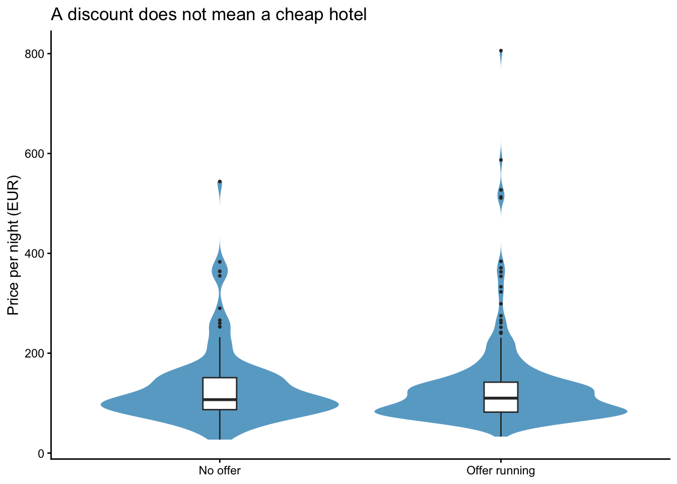

Figure 1: Price distribution with and without a discount offer running.

The reason is visible in the star column: discounted hotels carry a median of 3.5 stars against 3 for the others. Slightly better hotels discount slightly more often, and the two effects cancel.

The practical lesson — for a price comparison site, or for our own pricing — is that “on offer” carries essentially no information about what you will pay. It is a marketing label, not a statement about price.

Why this is a good answer

It asks something the board did not, reports a null result honestly instead of hunting for a difference, backs it with a second view of the data, and offers a mechanism. Null results are findings. Do not hide them.

6 If you finish early

6.1 a) Does a good rating command a bigger premium in the centre?

only_hotels |>
  filter(!is.na(rating)) |>
  mutate(
    wide_band  = cut(distance, c(-0.1, 1, 2, 100),
                     labels = c("<1 km", "1-2 km", ">2 km")),
    well_rated = if_else(rating >= 4.2, "rated 4.2+", "rated below 4.2")
  ) |>
  group_by(wide_band, well_rated) |>
  summarise(n = n(), median_price = median(price), .groups = "drop") |>
  ft()

wide_band	well_rated	n	median_price
<1 km	rated 4.2+	65	158.0
<1 km	rated below 4.2	61	108.0
1-2 km	rated 4.2+	20	102.5
1-2 km	rated below 4.2	56	82.0
>2 km	rated 4.2+	13	100.0
>2 km	rated below 4.2	37	80.0

The same structure appears as with stars. Within one kilometre of the centre a well-rated hotel charges a premium of €50. Beyond that the premium collapses to about €20.50 at one to two kilometres and €20 further out.

So the premium a good reputation commands is roughly 2.5 times as large in the centre as on the outskirts. Two variables interacting again — and again, doing this by hand means one table per combination.

With three variables we would need a dozen tables and most cells would hold a handful of hotels. That is the practical ceiling of this approach, and the reason session 8 exists.

6.2 b) The same pipeline without the pipe

Here is the Q1 pipeline written the way you would have had to write it before the pipe existed — as nested function calls:

arrange(
  summarise(
    group_by(hotels_clean, accommodation_type),
    n = n(),
    median_price = median(price),
    .groups = "drop"
  ),
  desc(median_price)
) |>
  ft()

accommodation_type	n	median_price
Apartment	124	133.0
Apart-hotel	4	120.5
Bed and breakfast	4	117.0
Vacation home Condo	2	111.5
Hotel	253	103.0
Pension	16	90.5
Guest House	8	72.5
Hostel	6	50.5

It produces exactly the same table. The difference is entirely in how it reads.

Which one would you rather find in six months?

The nested version has to be read inside out: find the innermost call (group_by), then work outwards to summarise, then to arrange. The order you read in is the reverse of the order things happen, and the argument that belongs to arrange (desc(median_price)) ends up nine lines away from the function it belongs to.

The piped version reads in the order the work happens, top to bottom. With three steps the nested version is merely annoying; with six it is genuinely hard to follow, and it is very easy to close a bracket in the wrong place.

This is the whole argument for the pipe. It changes nothing about what R does — it changes what you can read.

6.3 c) `round()` versus `floor(x + 0.5)`

tier_compare <- hotels_clean |>
  mutate(
    tier_up = factor(floor(stars + 0.5), levels = 1:5, labels = paste(1:5, "stars")),
    tier_rd = factor(round(stars),       levels = 1:5, labels = paste(1:5, "stars"))
  )

tier_compare |>
  count(tier_up, tier_rd, .drop = FALSE) |>
  filter(n > 0) |>
  ft()

tier_up	tier_rd	n
1 stars	1 stars	1
2 stars	2 stars	47
3 stars	2 stars	5
3 stars	3 stars	134
4 stars	4 stars	195
5 stars	4 stars	8
5 stars	5 stars	27

13 of the 417 properties end up in a different tier depending on which rounding rule you use. They are exactly the ones sitting on a half star:

tier_compare |>
  filter(tier_up != tier_rd) |>
  count(stars, tier_up, tier_rd) |>
  ft()

stars	tier_up	tier_rd	n
2.5	3 stars	2 stars	5
4.5	5 stars	4 stars	8

The 5 hotels rated 2.5 stars and the 8 rated 4.5 stars are pushed down a tier by round(), while the 3.5-star hotels are pushed up by both rules and so do not appear here at all.

left_join(
  count(tier_compare, tier_up, name = "floor_half_up"),
  count(tier_compare, tier_rd, name = "round_R") |> rename(tier_up = tier_rd),
  by = "tier_up"
) |>
  ft()

tier_up	floor_half_up	round_R
1 stars	1	1
2 stars	47	52
3 stars	139	134
4 stars	195	203
5 stars	35	27

Why this is worth knowing

The two rules disagree about 13 properties out of 417 — under 4%, and easy to dismiss. But look at where they land: round() shrinks the five-star tier from 35 to 27 properties, a drop of about 22.9%.

The five-star tier is the smallest and the most expensive. Losing eight of its members to the tier below moves both medians, and nothing in the output would have told you that a rounding rule was the cause.

The deeper point: round() is not wrong, it is inconsistent for this purpose — 2.5 and 4.5 go down while 3.5 goes up. Any rule is defensible as long as you know which one you chose. Choosing by accident is not.